Project Overview
This project utilized Eureqa — a symbolic regression and machine learning tool — to estimate vehicle speeds in the vicinity of traffic bottlenecks. Models use free-flow speed S, observed flow Q, and density K as inputs to predict speed V before, at, and after bottlenecks. The models achieve high explanatory power (R² > 0.97) and can be used for traffic planning, simulation and real-time control.
Average free speed
63.83 km/h
Speed before
9.84 km/h
Speed at bottleneck
31.91 km/h
Speed after
56.05 km/h
Model Visualizations
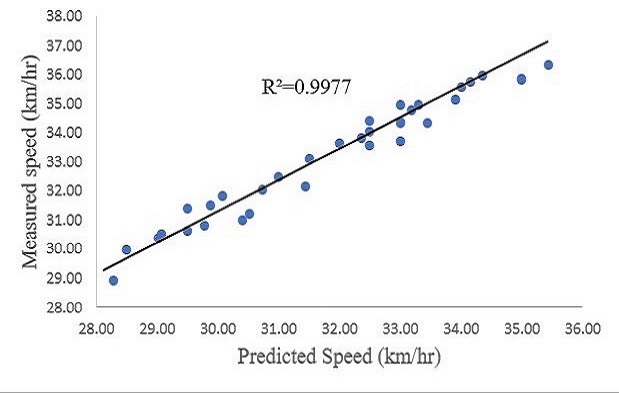
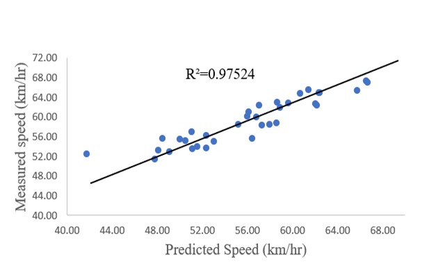
(ion.)
Data & Models
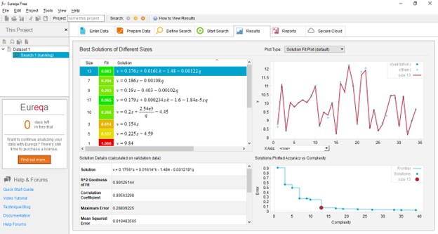
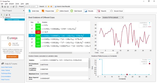
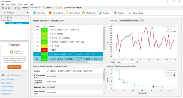
Models were derived using symbolic regression in Eureqa. Inputs: S = free speed (km/h), K = density (veh/km), Q = observed flow (veh/hr). Model fit statistics (R²) indicate very strong predictive power across all three stages.
Before bottleneck:
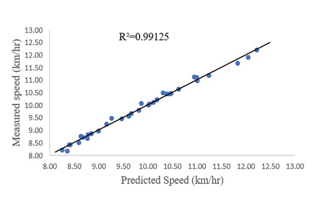
V = 0.176*S + 0.016*K - 1.48 - 0.00122*Q

At bottleneck:
V = 0.521*S + 0.000887*Q - 1.61 - 1.02e-5 * S*Q - 5.54e-8 * Q^2

After bottleneck:
V = 0.992*S + 0.439*K - 38.71 - 1.29e-6 * Q^2 - 0.00127 * K^2
Model performance (R²): Before 0.99125 • At 0.9977 • After 0.97524
Key Insights
- Sharp pre-bottleneck deceleration — vehicles reduce speed ~200–300 m before the critical point, typically due to roadside activities and boarding/alighting behavior.
- Severe speed drop at bottleneck — the narrow bottleneck segment shows the lowest mean speeds (~31.9 km/h), confirming queue formation at local chokepoints.
- Non-linear recovery after bottleneck — speed recovery follows an exponential-like trend; full normalization occurs around ~500 m downstream in typical conditions.
- High explanatory power — R² > 0.97 for all models indicates robust models suitable for planning and near real-time estimation.
- Density thresholds — jam density observed ≈ 282 veh/km; beyond this the flow relationship becomes unstable and delays increase drastically.
Recommendations
- Embed models into traffic control — integrate the equations into a simple tool (Excel, Python script or microservice) to estimate speeds in planning scenarios and trigger adaptive signal timings.
- Early-warning & driver advisory — use predicted pre-bottleneck deceleration to provide advance warnings to drivers (VMS or in-vehicle alerts) and recommend speed harmonization.
- Targeted infrastructure fixes — prioritize interventions (bus bay relocation, formalized loading areas, pedestrian crossings) at identified 100–300m approach zones to remove root causes.
- Real-time data fusion — combine sensor or probe-vehicle live data to re-run predictions and adjust control in near real-time, improving robustness during high-flow events.
- Use models for construction planning — apply the models to estimate travel-time impacts caused by temporary works and plan diversions or off-peak executions.
Impact
Deploying these models helps reduce delays, improve travel-time reliability, and supports evidence-based decisions for targeted investments (e.g., bus stop relocation, lane management). The models also serve as an educational tool for students and practitioners to explore speed–flow–density interactions.
Contact
+234 810 6326 897